Z-Domain Analysis
One thing I really feel was lacking in my education was a good treatment of Z-domain circuits and analysis. Although, maybe it wasn’t lacking and I just didn’t appreciate the applications of it. Either way, over time in my career I’ve had to develop my skills at Z-domain analysis and learn various tips and tricks to help approach the analysis in an intuitive way. It’s one thing to know how to apply an equation, but another to understand why you are applying the equation. My goal with this post is to highlight some of the important topics I think are useful for any Z-domain circuit and system analysis.
At the end of the day, the whole motivation for this post is contained in the Poles and Zeros section so feel free to skip to that if the earlier content is something you’ve seen before!
Tabe of Contents
Z-Domain Basics
Continuous time signals can be converted into a complex frequency domain by means of the Laplace Transform. For analog engineers, this is our domain of choice. Working in the s-domain provides deeper insights into circuit operation than time domain allows. This concept can be extended to discrete-time (aka sampled time) signals by means of the Z-Transform.
In my mind, the most intuitive way to compare the s-domain to the Z-domain is to think about an integrator. We know that in the s-domain this is represented simply as $\frac{1}{s}$ and know that for a constant input, the output will ramp up indefinitely. We are, of course, integrating. But what does this look like in the z-domain? What does it mean to integrate a sampled signal?
The conversion from the time domain and sampled-time domain requires us to re-frame how we think of time. In continuous time (which is the world we live in), time is always increasing and can be reduced to arbitrary levels of accuracy. Continuous time is uncountably infinite. Sampled-time, on the otherhand, has a strict step-size dictated by some periodic sampling signal. Each step-size, therefore, is well-definied meaning sampled-time is countably infinite.
Now, if we chop up or constant input into small discrete points instead of having an input that looks like $x(t) = 1$ in the time domain, we’d have $x[n] = 1$. This may look the same, but there is a subtle difference: $n$ is discrete. The next value of $n$ will be a pre-determined distance away from the previous value. The $M^{th}$ value of $n$ will be M-times that pre-determined step size from your starting value. And so-on. Now think about that in the context of integration. That step size is analogous to our $dx$ in the continuous-time equation $y(t) = \int x(t) dx$. So if we know the step size, to integrate we just need to add the current value of $x[n]$ to the previous value of $y[n]$. In otherwords, at any sampled-time value we know that the current integration value can be defined as $y[n] = x[n] + y[n-1]$. Extending that to arbitrary sizes, we can say:
++y[N] = \sum_{n=0}^{N} x[n]++
The key takeaway here is that since the interval is well-defined in sample-space, a sum performs the same function that integration does in the time-domain.
Now we have to look at this in the z-domain. We know that integration in the time-domain is represented as $\frac{1}{s}$, as mentioned earlier, so how can we transform the sampled-time version into a Z-domain expression?
Let’s start with the generic equation
++y[n] = x[n] + y[n-1]++
We want to find an expression $Y(z)$ for an input $X(z)$. That means we must convert those discrete time signals into Z-domain expressions. Two very simple relations are all we need for this (going any deeper than this is well beyond the scope of this post):
++\delta[n] \rightarrow 1++
++\delta[n-a] \rightarrow z^{-a}++
That yields:
++Y(z) = X(z) + Y(z)\cdot x^{-1}++
++\frac{Y(z)}{X(z)} = \frac{1}{1-z^{-1}}++
This result is equivalent to integration.
Conversion to Frequency Domain
Converting to the frequency domain requires a relation between the variable $z$ and frequency. Much like how the Laplace transform maps time to a complex frequency plane, the Z-Transform does something similar. Instead of a complex plane, however, it maps to a unit circle. I could go into more detail here, but suffice to say that when we map to a unit circle the outcome is that:
++z = e^{j\omega T}++
Where $T$ in this context is the sampling period. In general, analyzing a system with $T=1s$ simplifies things a bit without losing information.
So, using our integration example above let’s convert to the frequency domain:
++H(j\omega) = \frac{1}{1-e^{-j\omega}} = \frac{e^{j\omega}}{e^{j\omega} - 1}++
++H(j\omega) = \frac{\cos(\omega) + j\cdot \sin(\omega)}{\cos(\omega) - 1 + j\cdot \sin(\omega)} ++
Now we want to get the magnitude response so we will first multiple the numerator and denomonator by the complex conjugate of the denomonator.
++H(j\omega) = \frac{1}{4}\frac{1-\cos(\omega)-j\cdot \sin(\omega)}{\sin^2(\frac{\omega}{2})}++
To get the magnitude response we need to square the real an imaginary parts, sum them, and take the square root:
++H(\omega) = \frac{1}{2}\csc(\frac{\omega}{2})++
Obviously, getting the frequency response is a bit more labor-intensive than we’d like (I talk about an easier approach later). However we can now plot the response to see that it looks like it’s integrating (infinite gain at DC with a decreasing gain as frequency increases).
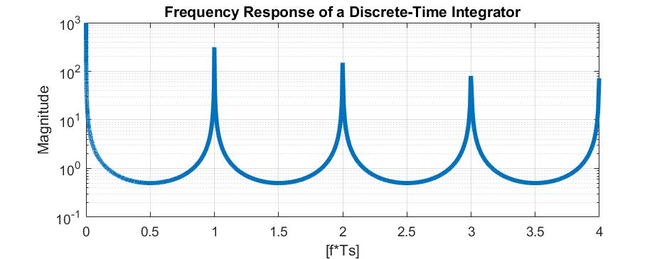
But that’s not quite true, is it? At every integer multiple of the sample frequency, the waveform again has infinite gain. This is an artifact of sampling. An intuitve way to thing about this is recall that we’re mapping the z-domain to a unit circle so unique values can only exist as we traverse the circumference of the circle once. We will see the same thing on the second revolution that we did on the first. Hence, every integer multiple of the sample frequency just means we’ve gone back to our starting point on the unit circle.
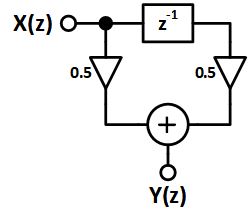
Simple Example
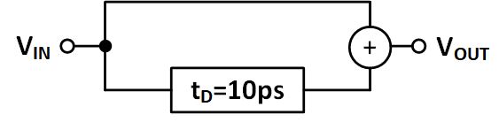
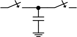
Let’s take a look at a simple example. See the diagram below. We have a signal that splits into two paths, one has a delay and the other does not. These lines are then summed before being output. As a sidenote, this example is actually part of an interview question I’ve been asked before and now ask when I’m interviewing. I think it’s a really good one that helps to figure out whether a candidate is comfortable with sampled systems (and if they’re not, it’s a really good way to see how they think about a problem and learn. Interview questions are somewhat useless if the candidate already knows the answer!).
We’re going to jump right into the thick of it and ask what happens if we have a sine wave entering the system and vary the frequency from 1Hz up to, say, 200GHz? Without an understanding of Z-transforms, good luck! But with our basic knowledge we’ve started to develop, we can limp through it.
We know that a delay element can be represented by $z^{-1}$ so all this system is doing is adding an input signal with a delayed version of that input signal. Thus:
++H(z) = 1 + z^{-1}++
From here we can insert $z = e^{j\omega T_s}$ and generate a frequency response (again, a more intuitive approach will be introduced later). For now, let’s just assume $T_s = 1$ despite the fact that the problem tells us what it is directly (we can add this in later).
++H(j\omega) = \frac{e^{j\omega} + 1}{e^{j\omega}}++
++H(j\omega) = \frac{\cos(\omega)+1+j\sin(\omega)}{\cos(\omega)+j\sin(\omega)}++
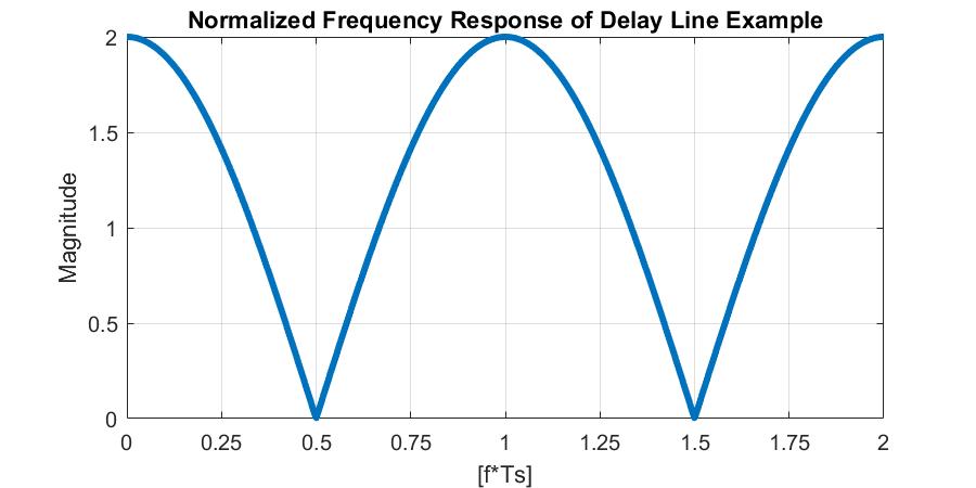
++H(\omega) = \sqrt{2}\sqrt{1+\cos(\omega)}++
If we were to plot this from $f = [0,2]$, we’d get the following graph
But since we’re given the delay of 10ps, we can simply muliple the x-axis by the inverse of that delay to get the actual frequency response:
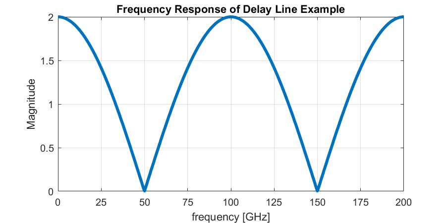
As a note, this type of system is typically refered to as a “Comb Filter” due to it’s shape (it kind of looks like a comb).
Switched Capacitor Circuits
In analog-land, Z-domain analysis is almost exclusively (perhaps entirely exclusively) used in conjunction with switched-capacitor circuits. This topic in itself is worthy of multiple blog posts, but I certainly don’t write like I’m running out of time (Alexander Hamilton anyone?) so that will perhaps never happen. However, we can scratch the surface.
Essentially, the idea behind switched capacitor circuits is that a resistor can be approximated by a capacitor that is periodically charged and held. The reason this is beneficial is that it can create very large resistors on an integrated circuit that would otherwise take up a lot of area: ie. it’s area-efficient.
Now imagine the first switch starts closed and the second switch starts open. Every $T_S$ seconds we will change the state of those switches. Also assume that the capacitor has a value $C_S$ and the input voltage is $V_{IN}$. If we apply a test current of $I_L$ at the output we can determine the resistance of this configuration.
At first, the charge on the capacitor will be $Q_C = V_{IN}C_S$. When the output switch opens, charge will be removed from the cap such that $Q_C = V_{IN}C_S - I_LT_S$. In otherwords:
++V_{OUT} = V_{IN} - \frac{I_LT_S}{C_S}++
Since we want to find the resistance, we have to put this equation in the form $\frac{V_{IN} - V_{OUT}}{I_L}$, therefore:
++R_{EFF} = \frac{T_S}{C_S} = \frac{1}{F_SC_S}++
So we can make a resistor by simply adjusting the sample period/frequency and the size of the capacitor. Beyond that, this concept is used beyond just making a resistor. Sampling a signal and holding it for some time is the basis of many ADC architectures. Processing charge by switching it between different capacitors is also a useful feature. As I said, this topic is large so I’m trying to make this is concise as possible.
Passive Filter
Now let’s apply the idea of a switched-capacitor resistor to an actual circuit we can use: a filter. We can quite easily construct a passive low-pass filter by replacing the resistor in a classic passive LPF with a switched-capactior version, like so:
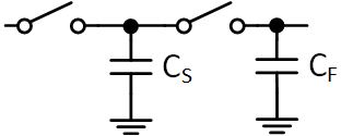
Up to around half of the sample frequency, it’s perfectly valid to say (provided $C_F \gg C_S$):
| ++ | H(s) | = \frac{1}{\sqrt{1+4\pi^2\frac{C_F}{C_S}fT_S}}++ |
However, given our knowledge of the Z-domain, we can improve upon this. Initially we know $Q_C[n-1] = V_{IN}C_S$. On the next phase, this charge is shared with $C_F$ such that:
++Q_{OUT}[n] = Q_C[n-1] + Q_F[n-1]++
The previous value of $Q_F$ must be $V_{OUT}C_F$ so plugging some expressions in we have:
++V_{OUT}[n] = V_{IN}\frac{C_S}{C_S+C_F} + V_{OUT}[n-1]\frac{C_F}{C_S+C_F}++
Converting to the Z-domain we get:
++H(z) = \frac{C_S}{C_S+C_F}\cdot\frac{1}{1-\frac{C_F}{C_S+C_F}z^{-1}}++
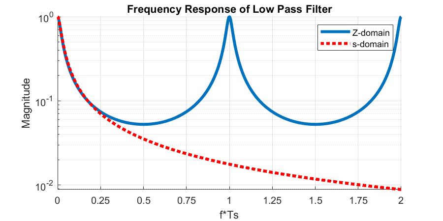
Which has the expected $\frac{1}{1-z^{-1}}$ structure for a low-pass filter. We can convert this into the frequency domain using similar methods as before and compare this to the continuous-time approximation (here, I’m setting $C_S=1F$ and $C_F=9F$ just for simplicity:
Demodulator
Another fun example is demodulating a periodic signal with switched capacitors. This demodulator is something I had the pleasure of working on at a previous job and is publically available as a patent: US5880411A.
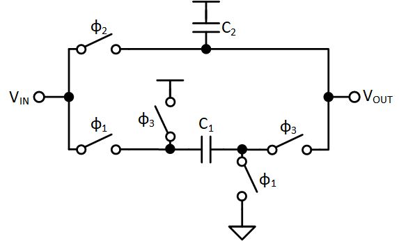
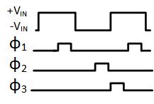
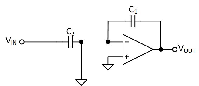
So let’s start to analyize this and, since we’re interested in the Z-domain, we’ll say the supply voltage is zero. First, let’s consider what the circuit looks like during $\phi_1$
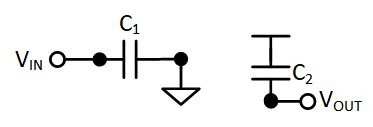
Here we are storing $V_{IN}$ on $C_1$ so our charge equations are:
++Q_1[n-1] = V_{IN}[n-1]C_1++
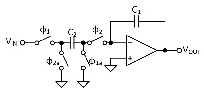
Next, let’s see what happens on $\phi_2$
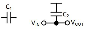
Here we can see that $C_1$ is floating, so there’s no change in the stored charge. $C_2$ sees $V_{IN}$ shorted to $V_{OUT}$ so (assuming the polarity of the capacitor is such that the positive side is connected to $V_{DD}$ which is zero in this example):
++Q_2[n] = -V_{IN}[n]C_2++
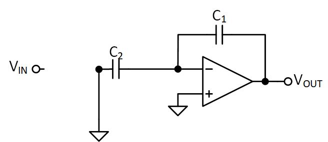
Finally, during $\phi_3$ the capacitors are shared (and note the polarity flip of $C_1$):
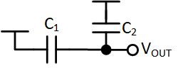
Due to the conservation of charge, we know the total charge previously stored on the capacitors must be the same as whatever the total charge is now. So:
++Q_{OUT}[n] = -V_{OUT}[n]\left(C_1+C_2\right)++
and, due to the polarity flip on $C_1$
++Q_{OUT}[n] = -Q_1[n-1] - Q_2[n]++
++V_{OUT}[n] = V_{IN}[n-1]\frac{C_1}{C_1+C_2} - V_{IN}[n]\frac{C_2}{C_1+C_2}++
++V_{OUT}(z) = V_{IN}(z)\frac{C_2}{C_1+C_2}\left(\frac{C_1}{C_2}z^{-1} - 1\right)++
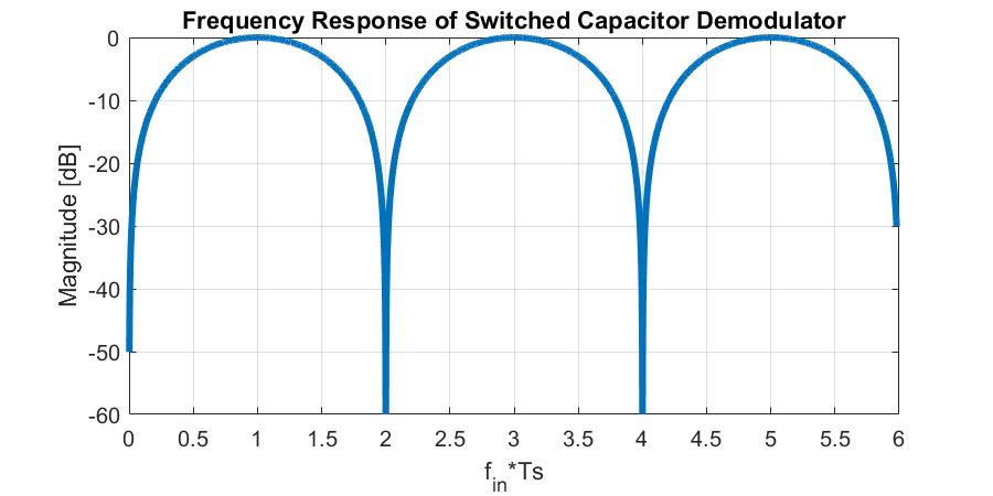
If we then convert this to the frequency domain and, for simplicity, assume $C_1 = C_2$ we can show that:
| ++ | H(j\omega) | = \frac{\sqrt{2}}{2}\sqrt{1-\cos(\omega)}++ |
If we plot this against the input frequency, noting that the sample frequency is 2x the input frequency, we can see that this demodulator circuit passes the odd harmonics of the signal and supresses the even harmonics.
Parasitic Insensitive Integrator (with finite gain)
Now let’s move on to probably the most common example of all time: the parasitic insensitive integrator. I’lll spare the details on the usefullness of being “parasitic insensitive” since I have nothing more to add to this subject that can’t be easily found in other material online. However, I’ll add a little twist that isn’t always talked about: the impact of finite amplifier gain.
Before we do the analysis, though, we should think about what we’d expect. An ideal integrator would have infinite gain at DC. So what about a non-ideal integrator? It’s fair to assume that at DC this gain would, instead, be finite. So when we plot the curves, we’d expect the gain to flatten out indiciating a pole at some low frequency.
Ok, let’s get on with it.
One simplification we’ll make is that $\phi_x$ and $\phi_{xa}$ are the same signal. In reality there’s some non-overlap added but that’s not required for our analysis. Like the previous example, let’s deconstruct the circuit to see what it looks like during each phase. For $\phi_1$ we have
First, it’s obvious that the charge on $C_2$ is
++Q_2[n-1] = V_{IN}[n-1]C_2++
Next, we have to think about what the inverting terminal voltage is. For an ideal op-amp, this would be whatever the non-inverting terminal is. But given that we’re considering a non-ideal amplifier, this approximation no longer holds. We know that $V_{OUT} = A_V\left(V_+ - V_-\right)$ so we can re-arrange this and, given that $V_+=0$ we know $V_- = -\frac{V_{OUT}}{A_V}$. This leaves us with:
++Q_1[n-1] = V_{OUT}[n-1]C_1(1+\frac{1}{A_V})++
Now let’s consider $\phi_2$
Here we know that, due to charge conservation, the charge from the previous phase must equal the total charge of this phase, or $Q_T[n] = Q_1[n-1] + Q_2[n-1]$. The total charge is:
++Q_T[n] = C_1V_{OUT}[n]\left(1+\frac{1}{A_V}\right) + C_2V_{OUT}[n]\frac{1}{A_V}++
So combining everything we get a transfer function of:
++H(z) = \frac{C_2}{C_1}\frac{1}{1+\frac{1}{A_V}}\cdot\frac{z^{-1}}{1+\frac{C_2}{C_1}\frac{1}{1+A_V}-z^{-1}}++
Notice the finite gain does two things. First, it reduces the total gain of the system. Second, it’s inclusion in the denominator indicates that it moves the pole frequency. If we think about the unit circle, the pole will move from $z=1$ and progress inwards. If we assume the gain cannot be negative, the minimum value would be $A_V=0$ which means that the pole could only move inwards to $z=\frac{1}{2}$, assuming $C_1=C_2$. Later on, we’ll deal with how knowing this can build intuition without doing any intensive math.
Now, if we assume that $A_V \rightarrow \infty$ and that $C_1=C_2$ we can see the ideal integrator equation pop out:
++H(z) = \frac{z^{-1}}{1-z^{-1}}++
So let’s go ahead and plot both the ideal and non-ideal equations. Again, we’ll assume $C_1=C_2$ and we’ll set $A_V=30\frac{V}{V}$
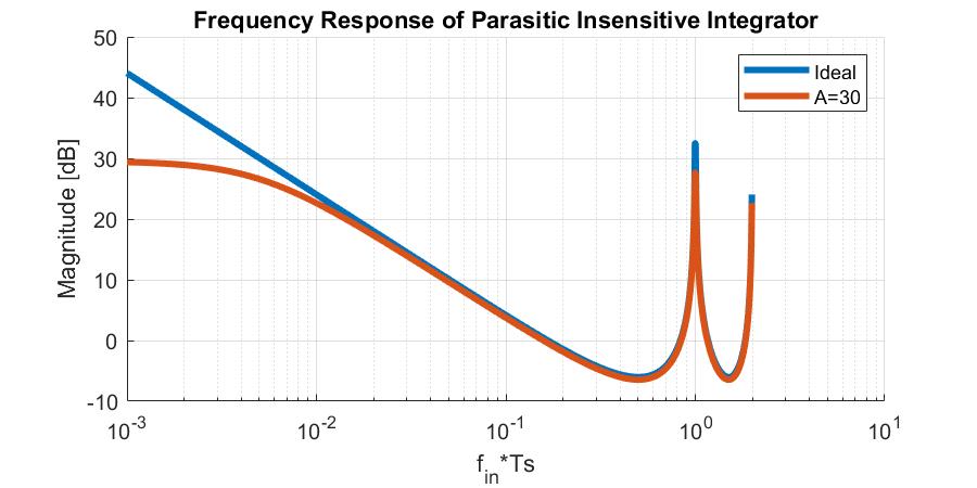
We can see that our earlier intutition is correct: the effect of finite gain is reduced gain at DC and an increased pole frequency.
First-order Delta Sigma Modulator
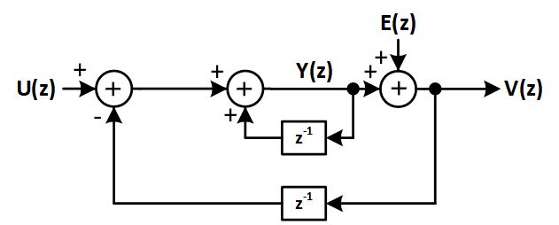
Our last example will be a first-order discrete-time $\Delta\Sigma$ modulator. I’m not going to dive into $\Delta\Sigma$ details here, so if you’re unfamiliar I’d recommend reading up on noise shaping data converters.
To start, we have a block diagram consisting of a integrator with a feedback loop wrapped around. At the output there is a “quantizer” (ie. an ADC… yes we’re building an ADC from an ADC) and an additional summing element where “quantization noise” can be injected. I’ve omitted the quantizer from this diagram because we’ll assume it’s ideal. Also, quantization noise is perhaps more aptly called “Quantization Error” since it is the error between the output digital signal and the input analog signal.
To begin analyzing this, let’s first consider the integrator. From earlier, we know that this configuration should result in the following transfer function:
++H(z) = \frac{1}{1-z^{-1}}++
From here we can just observe that the input to that integrator is the input signal $U(z)$ less a delayed version of the output signal $V(z)$ such that:
++Y(z) = U(z)H(z) - V(z)H(z)z^{-1}++
Assuming an ideal quantizer, we can also say that $Y(z) = V(z) - E(z)$ where $E(z)$ is the injected quantization noise. Solving for $V(z)$ yields:
++V(z) = U(z)\frac{H(z)}{1+H(z)z^{-1}} + E(z)\frac{1}{1+H(z)z^{-1}}++
Plugging in for $H(z)$ gives us:
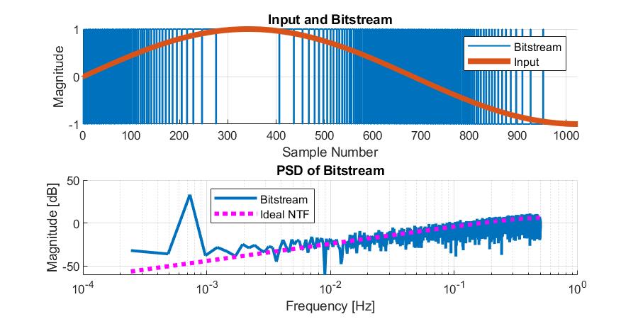
++V(z) = U(z) + E(z)\left(1-z^{-1}\right)++
What this tells us is that the output contains the original unfiltered signal along with a high-pass filtered version of the quantization noise. And because I find it more instructive to have an example, below is some MATLAB code you can use to “simulate” a simple $1^{st}$ order $\Delta\Sigma$. Note that the quantization noise is shaped accoriding to our expectation for the ideal “Noise Transfer Function”, or NTF.
%% dtdsmod1.m
%-------------------------------------
% Simple 1st order delta sigma model
% Author: Kevin Fronczak
% Date: 2020-16-07
%-------------------------------------

%% User variables
N = 2^12;       % Number of samples
Fs = 1;         % Sample Frequency
fin = 3*Fs/N;   % Input Frequency

%% Input signal generation
k = 0:1:(N-1);
u = sin(2*pi*fin*k);

%% Run DSM simulation
v = zeros(size(u));
y = zeros(size(u));
for n = 2:N
    y(n) = u(n) - v(n-1) + y(n-1);
    % Quantize the integrator output to [-1, 1]
    v(n) = -1;
    if y(n) >= 0.5
        v(n) = 1;
    end
end

%% Calculate PSD of bitstream
V = abs(fft(v));
V = V(1:N/2+1);
Vpsd = 2/(Fs*N)*V.^2;
Vpsd = 10*log10(Vpsd);
f = Fs*(0:(N/2))/N;

%% Get ideal NTF plot
NTF = tf([1 -1], [1 0], 1/Fs);
[ntf, ph, w] = bode(NTF, 2*pi*f);
ntf_psd(1,:) = 10*log10(ntf(1,1,:).^2);

%% Plot waveforms
figure(1)
subplot(2,1,1)
hold on;
stairs(k, v, 'LineWidth', 1)
stairs(k, u, 'LineWidth', 4)
hold off;
legend show;
legend({'Bitstream', 'Input'})
xlabel('Sample Number')
ylabel('Magnitude')
ylim([-1 1])
xlim([0 N/4])
title('Input and Bitstream')
grid on;

subplot(2,1,2)
hold on;
plot(f, Vpsd, 'LineWidth', 2)
plot(f, ntf_psd, ':m', 'LineWidth', 3)
hold off;
legend show;
legend({'Bitstream', 'Ideal NTF'}, 'location', 'SouthEast')
xlabel('Frequency [Hz]')
ylabel('Magnitude [dB]')
title('PSD of Bitstream')
set(gca, 'XScale', 'log')
grid on;
Poles and Zeros
Up to this point we really haven’t considered poles and zeros as far as a Z-domain equation is concerned. However, just like the s-domain, it’s pretty easy to find (set the numerator to zero, solve for z for zeros. For poles, do the same for the denominator). However, unlike the s-domain, the meaning of the poles and zeros is not immediately clear. For example, what does a pole at $z=0$ with a zero at $z=-1$ mean? If I asked you what the poles of an s-domain modeled looked like you’d likely be able to instantly relate that to frequency. The Z-domain version requires us to develop some intuition.
Estimating Frequency Response
Enter the unit circle. I alluded to it earlier, but the unit circle can be related to frequency by considering we traverse frequencies in the range of $0$ to $F_S$ as we travel counter-clockwise around the unit circle starting at $z=1$. So a zero at $z=-1$ means we’d expect the output of our system to go to zero at $\frac{F_S}{2}$. But what about that pole at $z=0$?
This is something that I, personally, didn’t learn until many years into my career. Which is a shame because it’s damn powerful.
Note that the example I’m highlighting is known as a 2-tap FIR filter, shown below. However, in the interest of keeping things simple I actually am ignoring the gain terms in the following analysis. However, since it is just a gain, all of the following plots can simply be scaled by $\frac{1}{2}$.
Now consider the following pole-zero plot:
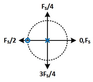
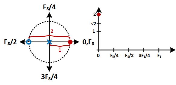
Now to figure out what happens in frequency we note that the magnitude is the distance you are from the zero, divided by the pole. For multiple poles and zeros, these are multipled. So let’s walk through this example.
To start, we’re at $f=0$. We are 2 units away from the zero and one away from the pole, giving us a magnitude of 2.
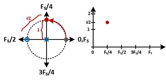
Next, we progress to $f=\frac{F_S}{4}$ at $z=j$. Here we need to use some trigonometry to figure out the distance we are from the zero. It should be relatively obvious that this means we are $\sqrt{2}$ away from the zero and 1 unit away from the pole so our value is now $\sqrt{2}$.
Now we’re at $f=\frac{F_S}{2}$. Here we are at the zero so the output is, well, zero.
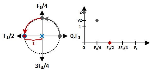
The next two frequencies are the same as $f=\frac{F_S}{4}$ and $f=F_S$, respectively. This results in the same plot we could get with complex analysis, yet uses only very simple math and builds intutition in terms of what poles and zeros mean in the Z-domain. For the record, if we ran through the $z=e^{j\omega T_S}$ analysis we’d get:
++\sqrt{2}\sqrt{1+\cos(\omega)}++
Developing Intuition
Now that we understand what’s happening with poles and zeros when placed on the unit circle, we can begin to develop some intuition in terms of what those poles and zeros do to the frequency response:
- Any zero on the unit circle will cause a null in the frequency response
- Any pole on the unit circle will cause the frequency response to be undefined (dividing by zero)
- As a zero moves from the unit circle towards the origin, the magnitude of the frequency response at that frequency will increase (ie. it’s no longer nulled)
- As a real pole increases from 0 to 1, the magnitude response at DC will increase and the response at $\frac{F_S}{2}$ will decrease
- As a real pole decreases from 0 to -1, the magnitude response at DC will decrease and the response at $\frac{F_S}{2}$ will increase
- In general, as poles move closer to the unit circle, the “peaks” are sharpened
- Poles outside the unit circle are treated similarly to RHP poles on an s-domain plot: they make the system unstable
4-tap FIR Filter
Now that we have some intuition, let’s extend the 2-tap FIR filter to a 4-tap FIR filter to see what happens.
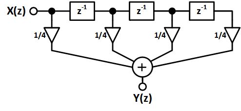
If we analyize this we’ll see that $Y(z) = \frac{1}{4}X(z)\left(1+z^{-1}+z^{-2}+z^{-3}\right)$. By extension, we can generalize an N-tap FIR filter to the following:
++Y_N(z) = \frac{1}{N}\left(1+\sum_{n}^{N-1} z^{-n}\right)++
If we solve the N=4 case for the poles and zeros, we can see we’ll end up with a pole at the origin and a total of three zeros: $z=-1$, $z=j$, and $z=-j$. Adding these to a pole-zero plot, we see:
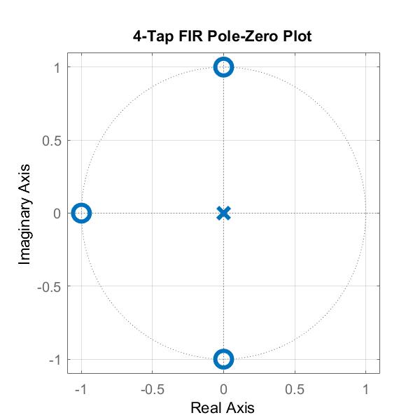
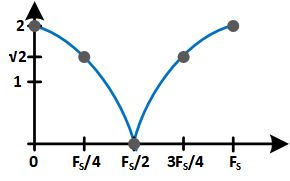
Now, let’s move around the unit circle and see what happens. This time we’ll make some intermediate stops since we can see there’s zeros at every multiple of $\frac{F_S}{4}$ which makes analysis less-than-interesting.
- f=0: $\frac{1}{4}\cdot\left(\frac{2}{1}\cdot\frac{\sqrt{2}}{1}\cdot\frac{\sqrt{2}}{1}\right)=\frac{1}{4}\cdot 4 = 1$
- f=Fs/8: using law of cosines $\frac{1}{4}\cdot\left(2+\sqrt{2}\right)\sqrt{2-\sqrt{2}}$
- f=Fs/4: $0$
- f=3/8Fs: $\frac{1}{4}\cdot\left(2-\sqrt{2}\right)\sqrt{2+\sqrt{2}}$
- f=Fs/2: $0$
- f=5/8Fs: $\frac{1}{4}\cdot\left(2-\sqrt{2}\right)\sqrt{2+\sqrt{2}}$
- f=3/4Fs: $0$
- f=7/8Fs: $\frac{1}{4}\cdot\left(2+\sqrt{2}\right)\sqrt{2-\sqrt{2}}$
- f=Fs: $1$
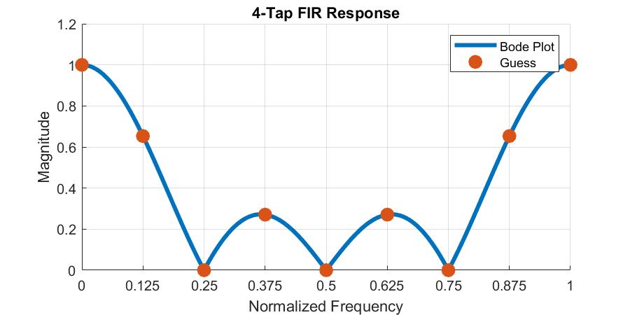
Plotting these values on top of the expected graph via MATLAB shows perfect alignment (and all it took was some light algebra):
Afterword
Using the pole-zero plot and traversing the unit circle is, in my opinion, a very powerful tool to quickly gain intuition in terms of what the frequency response of a system looks like. In many cases doing manual calculations is not needed and you can simply “mentally simulate” the circuit to gain insight. Using the 4-tap FIR as an example, we know for certain there are nulls at $\frac{F_S}{4}$, $\frac{F_S}{2}$, and $3\frac{F_S}{4}$. From there we might surmise that the magnitude response between the zeros is lower than at $0$ since the response must increase as it departs a zero and decrease as it approaches one. No trig or algebra required. Sure, we don’t get an exact value, but if we’re trying to gain some broad system level insight, those details aren’t needed (and can easily be extracted for us by MATLAB for when we do need them).
Hopefully I’ve been able to add a unique perspective to a topic I think is glossed over quite a bit! Thanks for reading!