Matched Filters
I came across a simple but interesting noise problem today dealing with the design of a matched filter. Matched filters, for those of you that may not know, are primarily used in communications systems and are meant to maximum the signal to noise ratio in a system (essentially they attempt to extract the most amount of signal and the least amount of noise). Wikipedia has a pretty decent explanation if you’re inclined to learn more. Basically, the problem is this: how can we design a matched filter to maximize the signal recovery? That is, how to we maximize our signal to noise ratio? Well, let’s take a look!
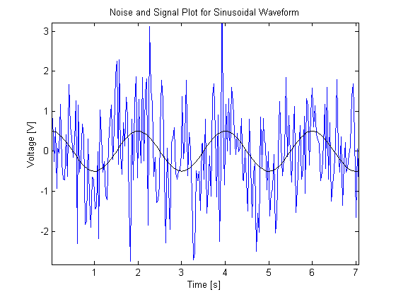
Let’s face it: we live in a very noisy world. No signal or waveform that we want to manipulate will ever be unaffected from noise in our environments. But how can we receive relatively clean signals when all this noise is around us? For an example, just take a look at the plot below! You can see what the signal should be: a nice, clean, sinusoidal waveform. But when we take into account noise, look at what happens- it’s barely discernible as a sine wave let alone a waveform at all! What can we do?!
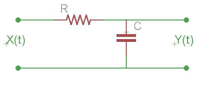
Well, let’s look at the background information we need first. Let’s say that the nice sine wave is the information we need to receive, but we end up getting all that blue stuff. Clearly, we need a way to filter all that noise out. There are many, many ways to do this, but let’s keep it simple and just pass our signal through a low-pass filter. Filter choice is largely dependent on the application, but let’s just pretend that a low pass filter will get us the information we want. Ok? Ok. First, we need to define what a low-pass filter is. We’ll just use a passive filter in order to simplify our calculations (and our ensuing transfer function). The circuit below is a low-pass filter (that is, it passes low frequencies while attenuating higher ones). Pretty easy so far!
Now, lets say we have a sinusoidal input defined as
++X(t)=A \cos{(\omega_{0} t+\Theta)}+N_{i}(t)++
where $N_{i}(t)$ is zero mean, white Gaussian noise. If you’re not sure what white Gaussian noise is, it’s simply noise that has the same amplitude across every frequency. Given we have white Gaussian noise, we know that the Power Spectral Density,
++S_{N_{i}}(f) = \frac{N_{0}}{2}++
This will be handy eventually, so just keep it in mind moving forward. First, let’s take a look what our signal to noise ratio, or $SNR_{i}$ is at the input of our filter. Since $SNR_{i} = \frac{Signal Power}{Noise Power}$ this is very easy to calculate.
For the sake of completeness, however, let’s find the power of our signal. How can we find this? By using the auto-correlation function! To find average power, we just take this function with $\tau = 0$ so we get:
++P_{avg}=R(0)=\frac{A^{2}}{2}++
How about the average power of the noise? Well, it happens to be $\infty$. Why? Well white Gaussian noise has a constant value across all frequencies so there is no autocorrelation between any points which results in $P_{avg}=R(0)=\infty$. That yields
++SNR_{i} = \frac{Signal Power}{Noise Power} = \frac{A^{2}/2}{\infty} = 0++
Wait, does that mean our noise has unlimited power?! Well, basically, all we have is noise. Eck. Enough of that, let’s start taking a look at our filter! First, we need to get the Transfer Function. Let’s start by taking the Fourier Transform of our circuit. This effectively only changes one component so now $C = \frac{1}{j\omega C}$. Now we can simply use voltage division to find our Transfer Function:
++ H(j\omega) = \frac{\frac{1}{j\omega C}}{R+\frac{1}{j\omega C}} H(j\omega) = \frac{1}{1+j\omega RC} ++
Now, let’s find the magnitude of this transfer function:
| ++ | H(j\omega) | = \frac{1}{\sqrt{1+\omega^{2}R^{2}C^{2}}}++ |
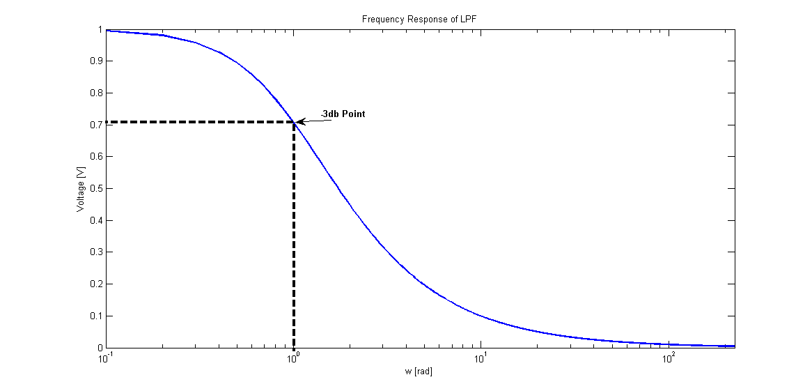
The next step we need to take is to find the -3dB point. This is the point where the signal starts to deteriorate at a -3dB/decade rate. Now, since this is a passive filter, we know the 0dB point is 1 and located at $\omega=0$. Therefore, we can find the -3dB point by solving for x in the follwoing equation:
$-3 = 20\log(x)$ which yields a value of $\frac{1}{\sqrt{2}}$
To help visualize this a bit better, refer to the following graph (ignore the x-axis values- they are arbitrary and were just used to help generate the plot):
So now that we have a magnitude value for our transfer function at the -3dB point, let’s solve for an expression in terms of R and C:
++\frac{1}{\sqrt{2}} = \frac{1}{\sqrt{1+\omega_{3db}^{2}R^{2}C^{2}}}
\frac{1}{2}+\frac{\omega_{3dB}^{2}R^{2}C^{2}}{2} = 1
\omega_{3db} = \frac{1}{RC}++
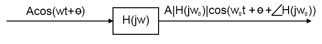
Now that we have all of that out of the way, we can start the design of our filter. First we need to determine what our output will look like after passing through our filter. This is illustrated in the figure below, but I’ll explain it as well. There are two things that the filter will do to our original signal. First, it will change the amplitude of the signal based on what the response is at a given frequency. The next is that it will have a phase change due to the phase at a given frequency.
We already know that the average Power of our input $X(t)$ is equal to $\frac{A^{2}}{2}$. Since out output will be scaled by the magintude of the Transfer Function we know that:
| ++P_{Y} = \frac{A^{2} | H(j\omega_{0}) | ^{2}}{2} = \frac{A^{2}}{2(1+\omega_{0}^{2}R^{2}C^{2})}++ |
Great! Now we have the output average power of our signal. Now, in order to get $SNR_{o}$ we just need to find the average output power of the noise. As discussed before, we know that the Power Spectral Density,
++S_{N_{i}}(\omega) = \frac{N_{0}}{2}++
As you might expect, the output is simply going to be scaled by the magnitude of the Transfer Function so
++ S_{N_{0}}(\omega) = S_{N_{0}}(\omega)|H(j\omega)|^{2}
= \frac{N_{0}}{2}\frac{1}{1+\omega^{2}R^{2}C^{2}} ++
To extract the average power from the Power Spectral Density, we simply multiply by $\frac{1}{2\pi}$ and integrate from $-\infty$ to $\infty$. This yields
++P_{N_{0}} = \frac{1}{2\pi}\int_{-\infty}^{\infty} S_{N_{0}}(\omega)\,d\omega= \frac{1}{2\pi}\int_{-\infty}^{\infty} \frac{N_{0}/2}{1+\omega^{2}R^{2}C^{2}},d\omega++
Now this certainly appears to be a rather tedious integral to calculate. However, if you recognize that
++\int \frac{dx}{1+ \alpha^{2}x^{2}} = \frac{1}{\alpha} = \tan^{-1}(\alpha x)++
and that we can say $\alpha = RC$ then our integral just became a whole lot simpler! Solving the integral leaves us with
| ++P_{N_{0}} = \left.\frac{N_{0}}{4\pi}\frac{1}{RC}\tan^{-1}(RC\omega_{0})\right | {-\infty}^{\infty} = \frac{N{0}}{4\pi RC}\left(\frac{\pi}{2}-\frac{-\pi}{2}\right) ++ |
Therefore, the average noise power at the output is given by: $\frac{N_{0}}{4RC}$. Now we can calculate $SNR_{o}$. Since this is just equal to $\frac{Signal Power}{Noise Power}$ we say
++SNR_{o} = \frac{\frac{A^{2}}{2(1+ \omega^{2} R^{2}C^{2})}}{\frac{N_0}{4 RC}}
=\frac{A^{2}}{2(1+ \omega^{2} R^{2}C^{2})}\cdot\frac{4 RC}{N_0}
= \frac{2 A^2}{N_0}\cdot\frac{RC}{1+ \omega^2 R^2 C^2}++
Now our goal is to design our filter to maximize $SNR$ so we need to take the derivative with respect to $RC$ and set that derivative equal to zero. To make our calculations a bit simpler, let’s set $x = RC$ so that
++SNR_0 = \frac{2 A^2}{N_0}\cdot\frac{x}{1+ \omega_{0}^{2} x^{2}}++
Now, we take the derivative:
++\frac{d(SNR_0)}{dx} =
\frac{2 A^2}{N_0}\cdot\frac{1+\omega_{0}^{2} x^{2} - 2 \omega_{0}^{2} x^{2}}{(1+\omega_{0}^{2} x^{2})^{2}} = 0++
Now we just need to solve for x.
++1+\omega_{0}^{2} x^{2} - 2 \omega_{0}^{2} x^{2} = 0 \Rightarrow \omega_{0}^{2} x^{2} = 1
\therefore RC = \frac{1}{\omega_{0}}++
Whoa! This result looks awfully familiar, doesn’t it? Remember when we found that $\omega_{3dB} = \frac{1}{RC}$? Well, we just found that in order to maximize our $SNR$ we should make the bandwidth of our filter equivalent to the 3dB bandwidth! Pretty neat, huh?! In that case, what is the best $SNR$ we can achieve with this configuration? Well, let’s solve for it!
++SNR_{max} = \frac{2A^2}{N_0}\cdot\frac{1/ \omega_0}{1+\omega_{0}^{2}\cdot \frac{1}{\omega_{0}^{2}}} = \frac{2A^{2}}{N_0}\cdot\frac{1/ \omega_0}{2}
\therefore SNR_{max} = \frac{A^2}{N_0 \omega_0}++
This actually tells us quite a bit about the system and how we can get the best signal to noise ratio. First, we must recognize that we have two variables to work with: the amplitude of the signal and the -3dB frequency (which is related to the frequency of our signal, as shown earlier). $ N_0$ is constant so we don’t really have to worry about it in this analysis. If we want the maximum signal to noise ratio, it’s pretty clear that increasing the amplitude (and thus the power) of our signal is the quickest way to success. However, increasing the amplitude, as just mentioned, increases the power of the signal which isn’t necessarily desirable or even an option. The next thing we could try is to lower our frequency. This, however, is very application dependent. The best design in this configuration would thus be to operate our signal at the lowest possible frequency while outputting at the highest allowed power. This will give us our best $SNR$ while still staying confined in our design parameters. Regardless, I thought this was a pretty neat problem to look at. It really illustrates the benefits of matched filters and how we can change our signal and filter in order to maximize signal recovery which, in communication systems at least, is absolutely vital. Hope you guys enjoyed this post (and hey, if you actually got to the end good on you!) and I’ll definitely post more neat theory-based problems like this whenever I spot a cool one. If you spot any mistakes, feel free to point it out in the comments. Thanks for reading!