Airplanes and Matrix Transformations

I’ve been busy (understatement of the year). I’ve been working on multiple projects (many of which will be highlighted here in the near future) and as the quarter is winding down, I figured I’d share some shorter ones I’ve worked on. This one is for a matrix class (essentially, the class focuses on the application of matrix theory- glorified linear algebra, if you will). The goal of this project was to construct a 3D object (an airplane) and perform various transforms on it. For all of the transformations that follow, green is the original aircraft while blue is the transformed version.

Now, let’s begin…

In order to perform matrix manipulations, three functions were created called rotate_3D, translate_3D, and dilate_3D. These functions, along with the script used to generate all of the following plots, can be found at the end of this document.

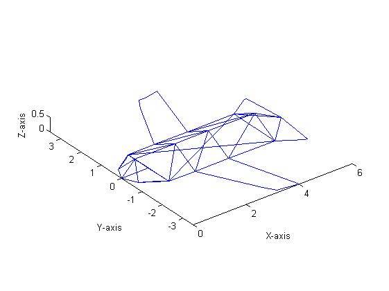
First, the aircraft shown in Figure 1 was dilated by 1.5. This was done by pre-multiplying the aircraft’s matrix (which can be a 3 x n sized matrix) by

++ \begin{bmatrix} 1.5 & 0 & 0 \ 0 & 1.5 & 0\ 0 & 0 & 1.5 \end{bmatrix}++

This resulted in Figure 2 (note that for all ensuing graphs, the blue aircraft is the transformation while the green is the original, unmodified, aircraft (as shown in Figure 1).

Next, the aircraft was reflected about the Y axis as shown in Figure 3. This was done by pre-multiplying the aircraft’s matrix by

++ \begin{bmatrix} -1 & 0 & 0 \ 0 & 1 & 0\ 0 & 0 & -1 \end{bmatrix}++

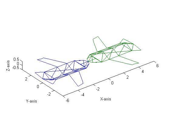
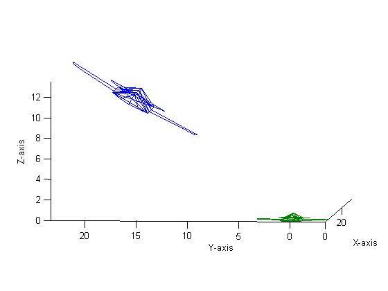
The aircraft then was rotated about the X axis by 60˚ (Figure 4). In order to perform a rotation in three-dimensional space, the following three matrices can be used:

++ R_{x} = \begin{bmatrix} 1 & 0 & 0 \ 0 & \cos{\alpha} & -\sin{\alpha}\ 0 & \sin{\alpha} & \cos{\alpha} \end{bmatrix} , R_{y} = \begin{bmatrix} \cos{\beta} & 0 & \sin{\beta} \ 0 & 1 & 0 \ -\sin{\beta} & 0 & \cos{\beta} \end{bmatrix} , R_{z} = \begin{bmatrix} \cos{\gamma} & -\sin{\gamma} & 0 \ \sin{\gamma} & \cos{\gamma} & 0\ 0 & 0 & 1 \end{bmatrix}++

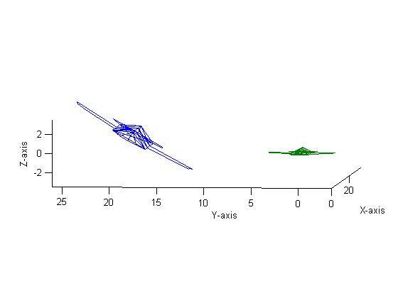
Where α is the roll angle, β is the pitch angle and ɣ is the yaw angle. Thus, a rotation of 60˚ about the X axis can also be called a roll of 60˚. Figure 5 shows a Yaw of 45˚, Figure 6 shows a Pitch of 30˚ and Figure 7 shows a Roll of 30˚.

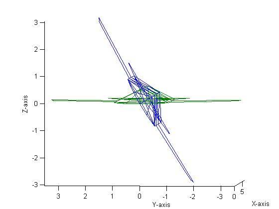
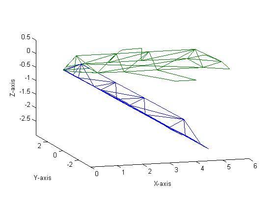
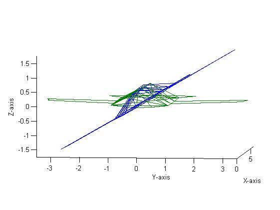
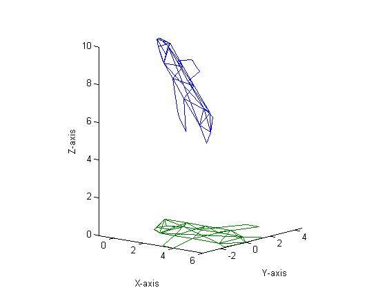
Figure 8 shows a translation by 10 units in the X direction, 10 units in the Y direction and 0 units in the Z direction followed by a rotation about the X-axis by 30˚ and finally a dilation of 2. The order was then changed to a rotation, translation and then dilation (all with the same parameters) which resulted in Figure 9. As one can see, the figures are clearly different. Mathematically, this makes sense and can be proven experimentally quite easily. Say we have a matrix

++A= \begin{bmatrix} 1 & 2 & 3 \ 2 & 3 & 4\ 1 & 0 & 1 \end{bmatrix}++

If we were to translate by 10 units in the X and Y direction and then rotate with a roll of 30˚ followed by a dilation of two, we would need to pre-multiply in the following order: DilationRotationTranslation*A. Thus, we can first multiply our Dilation and Rotation matrices:

++ D * R = \begin{bmatrix} 2 & 0 & 0 \ 0 & 2 & 0\ 0 & 0 & 2 \end{bmatrix} \begin{bmatrix} 1 & 0 & 0 \ 0 & \cos{30} & -\sin{30}\ 0 & \sin{30} & \cos{30} \end{bmatrix} = \begin{bmatrix} 2 & 0 & 0 \ 0 & 2\cos{30} & -2\sin{30}\ 0 & 2\sin{30} & 2\cos{30} \end{bmatrix} = \begin{bmatrix} 2 & 0 & 0 \ 0 & 1.73 & -1\ 0 & 1 & 1.73 \end{bmatrix}++

We can then take this matrix, which we’ll call C, and multiply it by our translation matrix T. However, in order to properly translate a matrix, we must increase the size from a 3 x3 to a 4 x4 by adding in a row vector of [0 0 0 1] and a column vector of [0 0 0 1]^T to the matrix C.

++M = CT = \begin{bmatrix} 2 & 0 & 0 & 0\ 0 & 1.73 & -1 & 0\ 0 & 1 & 1.73 & 0 \ 0 & 0 & 0 & 1\end{bmatrix} \begin{bmatrix} 1 & 0 & 0 & 10\ 0 & 1 & 0 & 10\ 0 & 0 & 1 & 0 \ 0 & 0 & 0 & 1\end{bmatrix} = \begin{bmatrix} 2 & 0 & 0 & 20\ 0 & 1.73 & -1 & 17.3\ 0 & 1 & 1.73 & 10 \ 0 & 0 & 0 & 1\end{bmatrix}++

We must now perform a row and column concatenation to our matrix A before pre-multiplying by M. We concatenate a row vector of [1 1 1 1] which represents the row’s scale value.

++B = MA = \begin{bmatrix} 2 & 0 & 0 & 20\ 0 & 1.73 & -1 & 17.3\ 0 & 1 & 1.73 & 10 \ 0 & 0 & 0 & 1\end{bmatrix} \begin{bmatrix} 1 & 2 & 3 & 0\ 2 & 3 & 4 & 0\ 1 & 0 & 1 & 0 \ 1 & 1 & 1 & 1\end{bmatrix} = \begin{bmatrix} 22 & 24 & 26 & 20\ 19.8 & 22.5 & 23.22 & 17.3\ 13.7 & 13 & 15.7 & 10 \ 1 & 1 & 1 & 1\end{bmatrix}++

If we change the order from Translate -> Rotate -> Dilate to Rotate -> Translate -> Dilate we would multiply as follows:

++B = DTRA = \begin{bmatrix} 2 & 0 & 0 & 0\ 0 & 2 & 0 & 0\ 0 & 0 & 2 & 0 \ 0 & 0 & 0 & 1\end{bmatrix} \begin{bmatrix} 1 & 0 & 0 & 10\ 0 & 1 & 0 & 10\ 0 & 0 & 1 & 0 \ 0 & 0 & 0 & 1\end{bmatrix} \begin{bmatrix} 1 & 0 & 0 & 0\ 0 & 0.866 & -0.5 & 0\ 0 & 0.5 & 0.866 & 0 \ 0 & 0 & 0 & 1\end{bmatrix} \begin{bmatrix} 1 & 2 & 3 & 0\ 2 & 3 & 4 & 0\ 1 & 0 & 1 & 0 \ 1 & 1 & 1 & 1\end{bmatrix} = \begin{bmatrix} 22 & 24 & 26 & 20\ 22.5 & 25.2 & 25.9 & 20\ 3.73 & 3 & 5.7 & 0 \ 1 & 1 & 1 & 1\end{bmatrix}++

Thus it is easy to see mathematically that the order of multiplications does, in fact, have an effect on the final matrix. This verifies the findings shown in Figures 8 and 9.

MATLAB CODE